Clustering of handwritten digits using Expectation-Maximization
For this project, We need to perform a soft clustering on these images using the Expectation-Maximization or EM algorithm.
What is the EM Algorithm?
We will need to revisit some concepts. Recall the different types of clustering methods-
- hard-clustering: clusters do not overlap, an element belongs to a cluster or it does not
- soft-clustering: clusters may overlap, an element may have 60% association with cluster 1 and 40% association with cluster 2
One way to envision these soft clusters is as two or more Gaussian probability distributions (Mixture models) with unknown parameters (Mean and Standard deviation).
Suppose we have data points coming from two different Guassian distributions and we are asked to calculate parameters of the 2 Gaussian sources.
library(ggplot2)
x <- rnorm(10, mean=2, sd=1)
y <- rnorm(10, mean=4, sd=1)
df <- data.frame(x,y)
ggplot(data=df) +
  geom_point(mapping=aes(x=x, y=0), col="blue") +
  stat_function(fun = dnorm, n = 101, args = list(mean = 2, sd = 1), col="blue") +
geom_point(mapping=aes(x=y, y=0), col="red") +
stat_function(fun = dnorm, n = 101, args = list(mean = 4, sd = 1), col="red")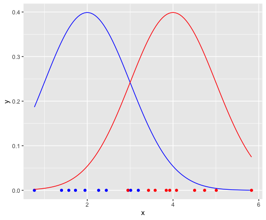
Given some points x, assumed to come from two unknown gaussian sources (a and b) how do we soft-cluster these points?
We need to calculate \(P(b|x_i) = \frac{P(x_i|b)P(b)}{P(x_i|b)P(b)+P(x_i|a)P(a)} \\\) For which we will need \(P(x_i|b) = \frac{1}{\sqrt{2\pi\sigma_b^2}}\exp(-\frac{(x_i-\mu_b)^2}{2\sigma_b^2}) \\\) To calculate this, we either need to know the Gaussian parameters or calculate sample mean and variance - which we can do only if we know which points belong to which distribution. As you can see, it’s quite tricky if we don’t have either of these. That’s where the EM algorithm comes in. This is an iterative process-
- We start with randomly placed Gaussians whose parameters are known
- E-step : For each point compute probability according to the first equation. The points can be re-clustered based on higher association
- M-step : From the new class membership, compute updated parameters to fit the points assigned
- Iterate until convergence
Let’s start by reading in the data - We have a dataset of 1593 handwritten digits which have been encoded in the form of Boolean variables based on the presence of a pixel in a 16x16 grayscale image. The first 256 columns are data and the 257th is the actual label for this training set.
rm(list=ls())
library(mvtnorm)
k =10
niter = 20
# Read handwritten digits data
myData=read.csv("semeion.csv",header=FALSE, sep=" ")
# Build data matrix with pixel and label data
myLabel=apply(myData[,257:266],1,function(xx){
  return(which(xx=="1")-1)
})
myX=data.matrix(myData[,1:256])
d = dim(myX)[2]
N = dim(myX)[1]
The initilization step uses k-means for hard-clustering. We obtain the starting cluster centers and initial class membership - gamma.
#initliaze values using kmeans
hwd_cluster = kmeans(myX, k, nstart = 30)
init_means = hwd_cluster$centers
cluster = hwd_cluster$cluster
init_cmp <- sapply(c(1:k), function(kk){
  return(dim(myX[cluster==kk,])[1]/N)
})
init_gammaik = matrix(0, N, k)
for (obs in c(1:length(cluster))) {
  init_gammaik[obs, cluster[obs]] = 1
}
Nk_init = colSums(init_gammaik)
pik_init = Nk_init/N
Since we are dealing with a large number of variables, we will use decomposition into Principle Components (testing of 0,2,4 and 6 PCs) for dimensionality reduction. An introductory explanation of PCA is available here.
We define the computeVariance function to calculate the sample variance during the M-step.
#function to compute covariance matrix
computeVariance <- function(kk,q) {
vc2 = matrix(0,d,d)
for (obs in c(1:N)) {
     vc1 = ((myX[obs,]-means[kk,])%*%t(myX[obs,]-means[kk,]))*gammaik[obs,kk]
     vc2 = vc2 + vc1
   }
   varcov = vc2/Nk[kk]
   if(q==0){
     myEig = eigen(varcov, symmetric = TRUE, only.values = TRUE)
     sigma_sq = sum(myEig$values[q+1:d], na.rm = TRUE)/(d-q)
     return(sigma_sq*diag(d))
   }
   myEig = eigen(varcov, symmetric = TRUE)
   Vq = myEig$vectors[,1:q]
   sigma_sq = sum(myEig$values[q+1:d], na.rm = TRUE)/(d-q)
   Wq = Vq%*%diag(sqrt(myEig$values[1:q]-sigma_sq))
   varcovk = Wq%*%t(Wq) + sigma_sq*diag(d)
   return(varcovk)
}

aics <- vector()
PCs = c(0,2,4,6)
obs_dll = matrix(0, length(PCs), niter)
labels = matrix(0, length(PCs), N)
qmeans = array(dim = c(length(PCs), k, d))
Looping over each of the PC values, we move into the E-step. Since we initialized cluster centers (means) and have the class membership (from which we can get variance using the above user-defined function), we can compute the prior and posterior probabilities to get the new class memberships. Given the updated class membership distribution, we move to M-step and compute parameter estimates and this goes on iteratively until convergence (we have set number of iterations to 20 at the start of this program but can impose a stopping condition as well).
# compute for each q
for (q in PCs) {
dll <- vector()
means = init_means
cmp = init_cmp
gammaik = init_gammaik
Nk = Nk_init
pik = pik_init
#iterate till convergence
for (iter in c(1:niter)) {
#Estep - compute current class membership probabilities
prob_density = sapply(c(1:k), function(kk){
return(pik[kk]*dmvnorm(myX, means[kk,], computeVariance(kk,q)))
})
gammaik = prob_density/rowSums(prob_density)
#record data log likelihood per iteration
dll <- append(dll,sum(log(rowSums(prob_density))))
#Mstep - given the current class membership distribution, compute parameter estimates
Nk = colSums(gammaik)
pik = Nk/N
for(i in c(1:k)){
means[i,] = colSums(sweep(myX, gammaik[,i], MARGIN = 1, '*'))/Nk[i]
}
}
idx = which(PCs==q, arr.ind = TRUE)
obs_dll[idx,] = dll
qmeans[idx,,] = means
# record AIC for each q
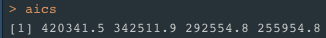
AIC = -2*tail(dll,1) + 2*(d*q + 1 - q*(q-1)/2)
aics = append(aics, AIC)
labels[idx,] = apply(gammaik, 1, function(xx){
return(which.max(xx)-1)
})
plot(dll, type = "l")
}The choice of number of Principal Components is based on the model with the lowest AIC(Akaike Information Criterion). It can be thought of as the model that explains most of the variability by using the smallest dimension of predictors.
We can also plot log-likelihood vs. iteration number to determine the best q (number of principle components).
#plot of data likelihood vs. iteration number
dev.new(width=6,height=6)
par(mar=c(0,0,0,0), mfrow=c(2,2))
for (i in c(1:dim(obs_dll)[1])){
  plot(obs_dll[i,], type="l")
}
Log likelihood is found to be highest and AIC lowest when q=6 so we go with number of PCs = 6 for our final model.
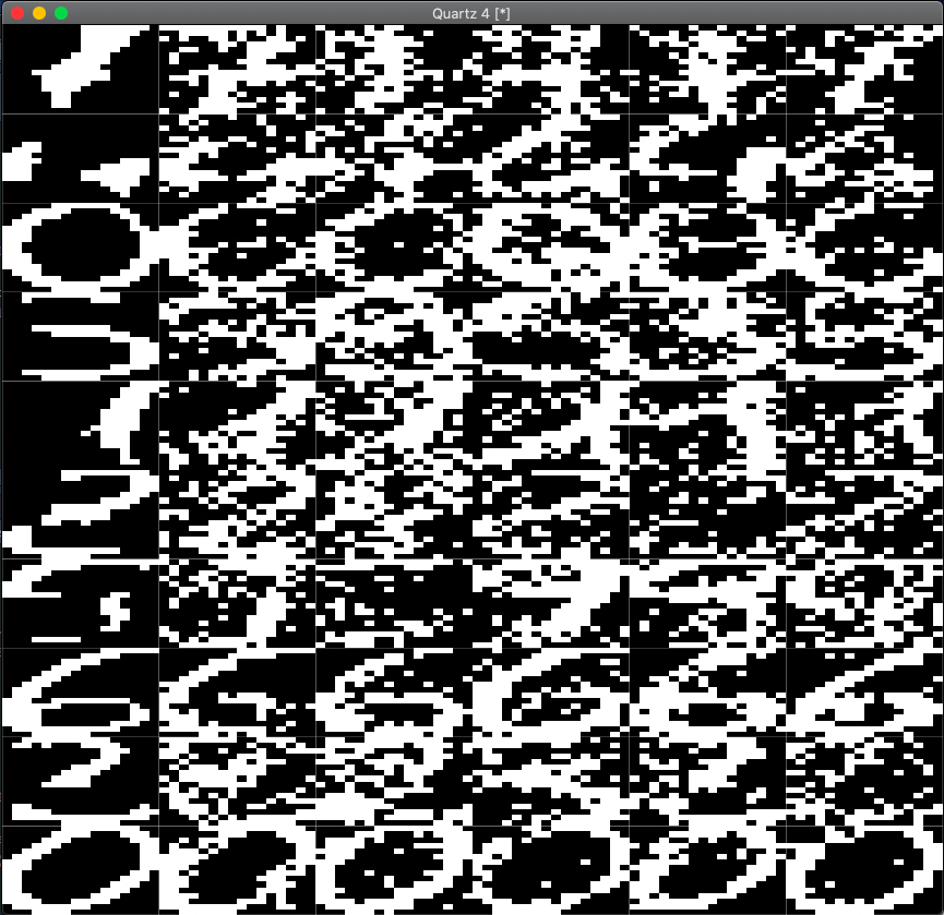
To observe how well the clustering model works and how well the cluster center is defined, we visualize 5 entries from each cluster formed along with their cluster centers -
#visualization
qchoice = PCs[which.min(aics)] #best q -> min AIC
idx = which(PCs==qchoice, arr.ind = TRUE)
newLabels = labels[idx,]
means = qmeans[idx,,]

dev.new(width=10,height=6)
par(mar=c(0,0,0,0), mfrow=c(10,6))
for(kk in c(1:k)) {
  image(t(matrix(means[kk,],byrow=TRUE,16,16)[16:1,]),col=gray(0:1),axes=FALSE)
  for(i in c(1:5)){
    img = rmvnorm(1, means[kk,], computeVariance(kk, qchoice))
    image(t(matrix(img,byrow=TRUE,16,16)[16:1,]),col=gray(0:1),axes=FALSE)
  }
  }
To evaluate the accuracy of our clustering, we identify the most occuring number in each of our clusters and evaluate how many were classified correctly (same as the identified number).
#calculating the miscategorization rate

groups = split(myLabel, newLabels)
miscategorizeRate = sapply(groups, function(grp){
  mcd = as.numeric(names(which.max(table(grp))))
  return(c(mcd, 1-(length(grp[grp==mcd])/length(grp))))
})
library(knitr)
kable(miscategorizeRate, col.names = c("Most common digit", "Miscategorization Rate"))

total_correct = sum(sapply(groups, function(grp){
  mcd = as.numeric(names(which.max(table(grp))))
  return(length(grp[grp==mcd]))
}))
overallMiscategorizeRate = 1-(total_correct)/N
print(overallMiscategorizeRate)
Miscategorization rate is found to be 33%. This is not too surprising as we do see that while 6 and 0 are usually identified correctly,some numbers like 5 and 4 are confused quite often with 9 and 7 respectively.
If you are looking for a simple explanation of the EM algorithm in a video format, I would recommend this lecture which I partially summarized in my explanation above. Thanks for reading!