Predict house prices with Linear Regression
This post was actually written in a Jupyter notebook (.ipynb) and converted to markdown format for posting on my github blog. I followed the instructions found here.
- Go to the location of your notebook.ipynb file using terminal and run jupyter nbconvert –to markdown notebook.ipynb. This will create notebook.md and notebook_files in the same directory
- Copy notebook.md to your _posts folder and contents of the notebook_files folder to your assets folder or wherever linked images are typically stored
- The notebook_files folder would contain plots and charts in PNG format which would need to be linked using the img src tag
- The CSS formatting mentioned in the post is quite important since the pandas dataframe tables may be unusual sizes. Make sure you set class=”dataframe” for every table if not already set so that the CSS formatting is applied.
Linear Regression is a supervised learning approach to predict a quantitative response. While it may be less exciting than modern statistical learning approaches, it serves as a good starting point for more sophisticated techniques and good understanding of this algorithm is crucial. It helps answer the question-
- Is there a relationship between the predictors and my dependent variable?
- How strong is this relationship and in what direction?
- How confident are we of this impact?
We will use the dataset obtained from this Kaggle competition - https://www.kaggle.com/c/house-prices-advanced-regression-techniques
Let’s start by reading in the dataset and looking at it’s contents.
import numpy as np
import pandas as pd

house_data = pd.read_csv('house-prices-advanced-regression-techniques/train.csv')
print(house_data.shape)
house_data.head()
(1460, 81)
| Id | MSSubClass | MSZoning | LotFrontage | LotArea | Street | Alley | LotShape | LandContour | Utilities | ... | PoolArea | PoolQC | Fence | MiscFeature | MiscVal | MoSold | YrSold | SaleType | SaleCondition | SalePrice | |
|---|---|---|---|---|---|---|---|---|---|---|---|---|---|---|---|---|---|---|---|---|---|
| 0 | 1 | 60 | RL | 65.0 | 8450 | Pave | NaN | Reg | Lvl | AllPub | ... | 0 | NaN | NaN | NaN | 0 | 2 | 2008 | WD | Normal | 208500 |
| 1 | 2 | 20 | RL | 80.0 | 9600 | Pave | NaN | Reg | Lvl | AllPub | ... | 0 | NaN | NaN | NaN | 0 | 5 | 2007 | WD | Normal | 181500 |
| 2 | 3 | 60 | RL | 68.0 | 11250 | Pave | NaN | IR1 | Lvl | AllPub | ... | 0 | NaN | NaN | NaN | 0 | 9 | 2008 | WD | Normal | 223500 |
| 3 | 4 | 70 | RL | 60.0 | 9550 | Pave | NaN | IR1 | Lvl | AllPub | ... | 0 | NaN | NaN | NaN | 0 | 2 | 2006 | WD | Abnorml | 140000 |
| 4 | 5 | 60 | RL | 84.0 | 14260 | Pave | NaN | IR1 | Lvl | AllPub | ... | 0 | NaN | NaN | NaN | 0 | 12 | 2008 | WD | Normal | 250000 |
5 rows × 81 columns
It is good practice to have at least 30 oberservations per variable and we see the need to cut down on number of predictors in our model (1438/81~18). One simple way to prune out less helpful predictors is to remove the ones with large number of missing values.
By observing the variable names as well as number of missing (NA) values, it is evident that the ones having ‘Garage’ or ‘Bsmt’ missing are observations for houses that do not have these features so they’re not actually missing, just not applicable.To make sure these stay in the dataset we choose our threshold as 6%.
#drop with more than 6% of missing values
house_data = house_data.loc[:, house_data.isna().mean()<0.06]
house_data.isna().sum().sort_values(ascending=False).head(20)
GarageType      81
GarageYrBlt     81
GarageFinish    81
GarageCond      81
GarageQual      81
BsmtExposure    38
BsmtFinType2    38
BsmtFinType1    37
BsmtCond        37
BsmtQual        37
MasVnrType       8
MasVnrArea       8
Electrical       1
RoofMatl         0
RoofStyle        0
SalePrice        0
Exterior1st      0
Exterior2nd      0
YearBuilt        0
ExterQual        0
dtype: int64
Another way to reduce number of variables as well as improve model quality is to keep only one from a group of correlated variables.I created a correlation matrix to identify correlated variables and mantained that one with higher correlation to sales.
corr_matrix = house_data.corr().style.apply(lambda x: ["background: red" if v > 0.7 or v < -0.7 else "" for v in x], axis = 1)
house_data = house_data.drop(['GarageYrBlt', 'GarageCars', 'TotRmsAbvGrd'], axis=1)
corr_matrix
| Id | MSSubClass | LotArea | OverallQual | OverallCond | YearBuilt | YearRemodAdd | MasVnrArea | BsmtFinSF1 | BsmtFinSF2 | BsmtUnfSF | TotalBsmtSF | 1stFlrSF | 2ndFlrSF | LowQualFinSF | GrLivArea | BsmtFullBath | BsmtHalfBath | FullBath | HalfBath | BedroomAbvGr | KitchenAbvGr | TotRmsAbvGrd | Fireplaces | GarageYrBlt | GarageCars | GarageArea | WoodDeckSF | OpenPorchSF | EnclosedPorch | 3SsnPorch | ScreenPorch | PoolArea | MiscVal | MoSold | YrSold | SalePrice | |
|---|---|---|---|---|---|---|---|---|---|---|---|---|---|---|---|---|---|---|---|---|---|---|---|---|---|---|---|---|---|---|---|---|---|---|---|---|---|
| Id | 1.000000 | 0.011156 | -0.033226 | -0.028365 | 0.012609 | -0.012713 | -0.021998 | -0.050298 | -0.005024 | -0.005968 | -0.007940 | -0.015415 | 0.010496 | 0.005590 | -0.044230 | 0.008273 | 0.002289 | -0.020155 | 0.005587 | 0.006784 | 0.037719 | 0.002951 | 0.027239 | -0.019772 | 0.000072 | 0.016570 | 0.017634 | -0.029643 | -0.000477 | 0.002889 | -0.046635 | 0.001330 | 0.057044 | -0.006242 | 0.021172 | 0.000712 | -0.021917 |
| MSSubClass | 0.011156 | 1.000000 | -0.139781 | 0.032628 | -0.059316 | 0.027850 | 0.040581 | 0.022936 | -0.069836 | -0.065649 | -0.140759 | -0.238518 | -0.251758 | 0.307886 | 0.046474 | 0.074853 | 0.003491 | -0.002333 | 0.131608 | 0.177354 | -0.023438 | 0.281721 | 0.040380 | -0.045569 | 0.085072 | -0.040110 | -0.098672 | -0.012579 | -0.006100 | -0.012037 | -0.043825 | -0.026030 | 0.008283 | -0.007683 | -0.013585 | -0.021407 | -0.084284 |
| LotArea | -0.033226 | -0.139781 | 1.000000 | 0.105806 | -0.005636 | 0.014228 | 0.013788 | 0.104160 | 0.214103 | 0.111170 | -0.002618 | 0.260833 | 0.299475 | 0.050986 | 0.004779 | 0.263116 | 0.158155 | 0.048046 | 0.126031 | 0.014259 | 0.119690 | -0.017784 | 0.190015 | 0.271364 | -0.024947 | 0.154871 | 0.180403 | 0.171698 | 0.084774 | -0.018340 | 0.020423 | 0.043160 | 0.077672 | 0.038068 | 0.001205 | -0.014261 | 0.263843 |
| OverallQual | -0.028365 | 0.032628 | 0.105806 | 1.000000 | -0.091932 | 0.572323 | 0.550684 | 0.411876 | 0.239666 | -0.059119 | 0.308159 | 0.537808 | 0.476224 | 0.295493 | -0.030429 | 0.593007 | 0.111098 | -0.040150 | 0.550600 | 0.273458 | 0.101676 | -0.183882 | 0.427452 | 0.396765 | 0.547766 | 0.600671 | 0.562022 | 0.238923 | 0.308819 | -0.113937 | 0.030371 | 0.064886 | 0.065166 | -0.031406 | 0.070815 | -0.027347 | 0.790982 |
| OverallCond | 0.012609 | -0.059316 | -0.005636 | -0.091932 | 1.000000 | -0.375983 | 0.073741 | -0.128101 | -0.046231 | 0.040229 | -0.136841 | -0.171098 | -0.144203 | 0.028942 | 0.025494 | -0.079686 | -0.054942 | 0.117821 | -0.194149 | -0.060769 | 0.012980 | -0.087001 | -0.057583 | -0.023820 | -0.324297 | -0.185758 | -0.151521 | -0.003334 | -0.032589 | 0.070356 | 0.025504 | 0.054811 | -0.001985 | 0.068777 | -0.003511 | 0.043950 | -0.077856 |
| YearBuilt | -0.012713 | 0.027850 | 0.014228 | 0.572323 | -0.375983 | 1.000000 | 0.592855 | 0.315707 | 0.249503 | -0.049107 | 0.149040 | 0.391452 | 0.281986 | 0.010308 | -0.183784 | 0.199010 | 0.187599 | -0.038162 | 0.468271 | 0.242656 | -0.070651 | -0.174800 | 0.095589 | 0.147716 | 0.825667 | 0.537850 | 0.478954 | 0.224880 | 0.188686 | -0.387268 | 0.031355 | -0.050364 | 0.004950 | -0.034383 | 0.012398 | -0.013618 | 0.522897 |
| YearRemodAdd | -0.021998 | 0.040581 | 0.013788 | 0.550684 | 0.073741 | 0.592855 | 1.000000 | 0.179618 | 0.128451 | -0.067759 | 0.181133 | 0.291066 | 0.240379 | 0.140024 | -0.062419 | 0.287389 | 0.119470 | -0.012337 | 0.439046 | 0.183331 | -0.040581 | -0.149598 | 0.191740 | 0.112581 | 0.642277 | 0.420622 | 0.371600 | 0.205726 | 0.226298 | -0.193919 | 0.045286 | -0.038740 | 0.005829 | -0.010286 | 0.021490 | 0.035743 | 0.507101 |
| MasVnrArea | -0.050298 | 0.022936 | 0.104160 | 0.411876 | -0.128101 | 0.315707 | 0.179618 | 1.000000 | 0.264736 | -0.072319 | 0.114442 | 0.363936 | 0.344501 | 0.174561 | -0.069071 | 0.390857 | 0.085310 | 0.026673 | 0.276833 | 0.201444 | 0.102821 | -0.037610 | 0.280682 | 0.249070 | 0.252691 | 0.364204 | 0.373066 | 0.159718 | 0.125703 | -0.110204 | 0.018796 | 0.061466 | 0.011723 | -0.029815 | -0.005965 | -0.008201 | 0.477493 |
| BsmtFinSF1 | -0.005024 | -0.069836 | 0.214103 | 0.239666 | -0.046231 | 0.249503 | 0.128451 | 0.264736 | 1.000000 | -0.050117 | -0.495251 | 0.522396 | 0.445863 | -0.137079 | -0.064503 | 0.208171 | 0.649212 | 0.067418 | 0.058543 | 0.004262 | -0.107355 | -0.081007 | 0.044316 | 0.260011 | 0.153484 | 0.224054 | 0.296970 | 0.204306 | 0.111761 | -0.102303 | 0.026451 | 0.062021 | 0.140491 | 0.003571 | -0.015727 | 0.014359 | 0.386420 |
| BsmtFinSF2 | -0.005968 | -0.065649 | 0.111170 | -0.059119 | 0.040229 | -0.049107 | -0.067759 | -0.072319 | -0.050117 | 1.000000 | -0.209294 | 0.104810 | 0.097117 | -0.099260 | 0.014807 | -0.009640 | 0.158678 | 0.070948 | -0.076444 | -0.032148 | -0.015728 | -0.040751 | -0.035227 | 0.046921 | -0.088011 | -0.038264 | -0.018227 | 0.067898 | 0.003093 | 0.036543 | -0.029993 | 0.088871 | 0.041709 | 0.004940 | -0.015211 | 0.031706 | -0.011378 |
| BsmtUnfSF | -0.007940 | -0.140759 | -0.002618 | 0.308159 | -0.136841 | 0.149040 | 0.181133 | 0.114442 | -0.495251 | -0.209294 | 1.000000 | 0.415360 | 0.317987 | 0.004469 | 0.028167 | 0.240257 | -0.422900 | -0.095804 | 0.288886 | -0.041118 | 0.166643 | 0.030086 | 0.250647 | 0.051575 | 0.190708 | 0.214175 | 0.183303 | -0.005316 | 0.129005 | -0.002538 | 0.020764 | -0.012579 | -0.035092 | -0.023837 | 0.034888 | -0.041258 | 0.214479 |
| TotalBsmtSF | -0.015415 | -0.238518 | 0.260833 | 0.537808 | -0.171098 | 0.391452 | 0.291066 | 0.363936 | 0.522396 | 0.104810 | 0.415360 | 1.000000 | 0.819530 | -0.174512 | -0.033245 | 0.454868 | 0.307351 | -0.000315 | 0.323722 | -0.048804 | 0.050450 | -0.068901 | 0.285573 | 0.339519 | 0.322445 | 0.434585 | 0.486665 | 0.232019 | 0.247264 | -0.095478 | 0.037384 | 0.084489 | 0.126053 | -0.018479 | 0.013196 | -0.014969 | 0.613581 |
| 1stFlrSF | 0.010496 | -0.251758 | 0.299475 | 0.476224 | -0.144203 | 0.281986 | 0.240379 | 0.344501 | 0.445863 | 0.097117 | 0.317987 | 0.819530 | 1.000000 | -0.202646 | -0.014241 | 0.566024 | 0.244671 | 0.001956 | 0.380637 | -0.119916 | 0.127401 | 0.068101 | 0.409516 | 0.410531 | 0.233449 | 0.439317 | 0.489782 | 0.235459 | 0.211671 | -0.065292 | 0.056104 | 0.088758 | 0.131525 | -0.021096 | 0.031372 | -0.013604 | 0.605852 |
| 2ndFlrSF | 0.005590 | 0.307886 | 0.050986 | 0.295493 | 0.028942 | 0.010308 | 0.140024 | 0.174561 | -0.137079 | -0.099260 | 0.004469 | -0.174512 | -0.202646 | 1.000000 | 0.063353 | 0.687501 | -0.169494 | -0.023855 | 0.421378 | 0.609707 | 0.502901 | 0.059306 | 0.616423 | 0.194561 | 0.070832 | 0.183926 | 0.138347 | 0.092165 | 0.208026 | 0.061989 | -0.024358 | 0.040606 | 0.081487 | 0.016197 | 0.035164 | -0.028700 | 0.319334 |
| LowQualFinSF | -0.044230 | 0.046474 | 0.004779 | -0.030429 | 0.025494 | -0.183784 | -0.062419 | -0.069071 | -0.064503 | 0.014807 | 0.028167 | -0.033245 | -0.014241 | 0.063353 | 1.000000 | 0.134683 | -0.047143 | -0.005842 | -0.000710 | -0.027080 | 0.105607 | 0.007522 | 0.131185 | -0.021272 | -0.036363 | -0.094480 | -0.067601 | -0.025444 | 0.018251 | 0.061081 | -0.004296 | 0.026799 | 0.062157 | -0.003793 | -0.022174 | -0.028921 | -0.025606 |
| GrLivArea | 0.008273 | 0.074853 | 0.263116 | 0.593007 | -0.079686 | 0.199010 | 0.287389 | 0.390857 | 0.208171 | -0.009640 | 0.240257 | 0.454868 | 0.566024 | 0.687501 | 0.134683 | 1.000000 | 0.034836 | -0.018918 | 0.630012 | 0.415772 | 0.521270 | 0.100063 | 0.825489 | 0.461679 | 0.231197 | 0.467247 | 0.468997 | 0.247433 | 0.330224 | 0.009113 | 0.020643 | 0.101510 | 0.170205 | -0.002416 | 0.050240 | -0.036526 | 0.708624 |
| BsmtFullBath | 0.002289 | 0.003491 | 0.158155 | 0.111098 | -0.054942 | 0.187599 | 0.119470 | 0.085310 | 0.649212 | 0.158678 | -0.422900 | 0.307351 | 0.244671 | -0.169494 | -0.047143 | 0.034836 | 1.000000 | -0.147871 | -0.064512 | -0.030905 | -0.150673 | -0.041503 | -0.053275 | 0.137928 | 0.124553 | 0.131881 | 0.179189 | 0.175315 | 0.067341 | -0.049911 | -0.000106 | 0.023148 | 0.067616 | -0.023047 | -0.025361 | 0.067049 | 0.227122 |
| BsmtHalfBath | -0.020155 | -0.002333 | 0.048046 | -0.040150 | 0.117821 | -0.038162 | -0.012337 | 0.026673 | 0.067418 | 0.070948 | -0.095804 | -0.000315 | 0.001956 | -0.023855 | -0.005842 | -0.018918 | -0.147871 | 1.000000 | -0.054536 | -0.012340 | 0.046519 | -0.037944 | -0.023836 | 0.028976 | -0.077464 | -0.020891 | -0.024536 | 0.040161 | -0.025324 | -0.008555 | 0.035114 | 0.032121 | 0.020025 | -0.007367 | 0.032873 | -0.046524 | -0.016844 |
| FullBath | 0.005587 | 0.131608 | 0.126031 | 0.550600 | -0.194149 | 0.468271 | 0.439046 | 0.276833 | 0.058543 | -0.076444 | 0.288886 | 0.323722 | 0.380637 | 0.421378 | -0.000710 | 0.630012 | -0.064512 | -0.054536 | 1.000000 | 0.136381 | 0.363252 | 0.133115 | 0.554784 | 0.243671 | 0.484557 | 0.469672 | 0.405656 | 0.187703 | 0.259977 | -0.115093 | 0.035353 | -0.008106 | 0.049604 | -0.014290 | 0.055872 | -0.019669 | 0.560664 |
| HalfBath | 0.006784 | 0.177354 | 0.014259 | 0.273458 | -0.060769 | 0.242656 | 0.183331 | 0.201444 | 0.004262 | -0.032148 | -0.041118 | -0.048804 | -0.119916 | 0.609707 | -0.027080 | 0.415772 | -0.030905 | -0.012340 | 0.136381 | 1.000000 | 0.226651 | -0.068263 | 0.343415 | 0.203649 | 0.196785 | 0.219178 | 0.163549 | 0.108080 | 0.199740 | -0.095317 | -0.004972 | 0.072426 | 0.022381 | 0.001290 | -0.009050 | -0.010269 | 0.284108 |
| BedroomAbvGr | 0.037719 | -0.023438 | 0.119690 | 0.101676 | 0.012980 | -0.070651 | -0.040581 | 0.102821 | -0.107355 | -0.015728 | 0.166643 | 0.050450 | 0.127401 | 0.502901 | 0.105607 | 0.521270 | -0.150673 | 0.046519 | 0.363252 | 0.226651 | 1.000000 | 0.198597 | 0.676620 | 0.107570 | -0.064518 | 0.086106 | 0.065253 | 0.046854 | 0.093810 | 0.041570 | -0.024478 | 0.044300 | 0.070703 | 0.007767 | 0.046544 | -0.036014 | 0.168213 |
| KitchenAbvGr | 0.002951 | 0.281721 | -0.017784 | -0.183882 | -0.087001 | -0.174800 | -0.149598 | -0.037610 | -0.081007 | -0.040751 | 0.030086 | -0.068901 | 0.068101 | 0.059306 | 0.007522 | 0.100063 | -0.041503 | -0.037944 | 0.133115 | -0.068263 | 0.198597 | 1.000000 | 0.256045 | -0.123936 | -0.124411 | -0.050634 | -0.064433 | -0.090130 | -0.070091 | 0.037312 | -0.024600 | -0.051613 | -0.014525 | 0.062341 | 0.026589 | 0.031687 | -0.135907 |
| TotRmsAbvGrd | 0.027239 | 0.040380 | 0.190015 | 0.427452 | -0.057583 | 0.095589 | 0.191740 | 0.280682 | 0.044316 | -0.035227 | 0.250647 | 0.285573 | 0.409516 | 0.616423 | 0.131185 | 0.825489 | -0.053275 | -0.023836 | 0.554784 | 0.343415 | 0.676620 | 0.256045 | 1.000000 | 0.326114 | 0.148112 | 0.362289 | 0.337822 | 0.165984 | 0.234192 | 0.004151 | -0.006683 | 0.059383 | 0.083757 | 0.024763 | 0.036907 | -0.034516 | 0.533723 |
| Fireplaces | -0.019772 | -0.045569 | 0.271364 | 0.396765 | -0.023820 | 0.147716 | 0.112581 | 0.249070 | 0.260011 | 0.046921 | 0.051575 | 0.339519 | 0.410531 | 0.194561 | -0.021272 | 0.461679 | 0.137928 | 0.028976 | 0.243671 | 0.203649 | 0.107570 | -0.123936 | 0.326114 | 1.000000 | 0.046822 | 0.300789 | 0.269141 | 0.200019 | 0.169405 | -0.024822 | 0.011257 | 0.184530 | 0.095074 | 0.001409 | 0.046357 | -0.024096 | 0.466929 |
| GarageYrBlt | 0.000072 | 0.085072 | -0.024947 | 0.547766 | -0.324297 | 0.825667 | 0.642277 | 0.252691 | 0.153484 | -0.088011 | 0.190708 | 0.322445 | 0.233449 | 0.070832 | -0.036363 | 0.231197 | 0.124553 | -0.077464 | 0.484557 | 0.196785 | -0.064518 | -0.124411 | 0.148112 | 0.046822 | 1.000000 | 0.588920 | 0.564567 | 0.224577 | 0.228425 | -0.297003 | 0.023544 | -0.075418 | -0.014501 | -0.032417 | 0.005337 | -0.001014 | 0.486362 |
| GarageCars | 0.016570 | -0.040110 | 0.154871 | 0.600671 | -0.185758 | 0.537850 | 0.420622 | 0.364204 | 0.224054 | -0.038264 | 0.214175 | 0.434585 | 0.439317 | 0.183926 | -0.094480 | 0.467247 | 0.131881 | -0.020891 | 0.469672 | 0.219178 | 0.086106 | -0.050634 | 0.362289 | 0.300789 | 0.588920 | 1.000000 | 0.882475 | 0.226342 | 0.213569 | -0.151434 | 0.035765 | 0.050494 | 0.020934 | -0.043080 | 0.040522 | -0.039117 | 0.640409 |
| GarageArea | 0.017634 | -0.098672 | 0.180403 | 0.562022 | -0.151521 | 0.478954 | 0.371600 | 0.373066 | 0.296970 | -0.018227 | 0.183303 | 0.486665 | 0.489782 | 0.138347 | -0.067601 | 0.468997 | 0.179189 | -0.024536 | 0.405656 | 0.163549 | 0.065253 | -0.064433 | 0.337822 | 0.269141 | 0.564567 | 0.882475 | 1.000000 | 0.224666 | 0.241435 | -0.121777 | 0.035087 | 0.051412 | 0.061047 | -0.027400 | 0.027974 | -0.027378 | 0.623431 |
| WoodDeckSF | -0.029643 | -0.012579 | 0.171698 | 0.238923 | -0.003334 | 0.224880 | 0.205726 | 0.159718 | 0.204306 | 0.067898 | -0.005316 | 0.232019 | 0.235459 | 0.092165 | -0.025444 | 0.247433 | 0.175315 | 0.040161 | 0.187703 | 0.108080 | 0.046854 | -0.090130 | 0.165984 | 0.200019 | 0.224577 | 0.226342 | 0.224666 | 1.000000 | 0.058661 | -0.125989 | -0.032771 | -0.074181 | 0.073378 | -0.009551 | 0.021011 | 0.022270 | 0.324413 |
| OpenPorchSF | -0.000477 | -0.006100 | 0.084774 | 0.308819 | -0.032589 | 0.188686 | 0.226298 | 0.125703 | 0.111761 | 0.003093 | 0.129005 | 0.247264 | 0.211671 | 0.208026 | 0.018251 | 0.330224 | 0.067341 | -0.025324 | 0.259977 | 0.199740 | 0.093810 | -0.070091 | 0.234192 | 0.169405 | 0.228425 | 0.213569 | 0.241435 | 0.058661 | 1.000000 | -0.093079 | -0.005842 | 0.074304 | 0.060762 | -0.018584 | 0.071255 | -0.057619 | 0.315856 |
| EnclosedPorch | 0.002889 | -0.012037 | -0.018340 | -0.113937 | 0.070356 | -0.387268 | -0.193919 | -0.110204 | -0.102303 | 0.036543 | -0.002538 | -0.095478 | -0.065292 | 0.061989 | 0.061081 | 0.009113 | -0.049911 | -0.008555 | -0.115093 | -0.095317 | 0.041570 | 0.037312 | 0.004151 | -0.024822 | -0.297003 | -0.151434 | -0.121777 | -0.125989 | -0.093079 | 1.000000 | -0.037305 | -0.082864 | 0.054203 | 0.018361 | -0.028887 | -0.009916 | -0.128578 |
| 3SsnPorch | -0.046635 | -0.043825 | 0.020423 | 0.030371 | 0.025504 | 0.031355 | 0.045286 | 0.018796 | 0.026451 | -0.029993 | 0.020764 | 0.037384 | 0.056104 | -0.024358 | -0.004296 | 0.020643 | -0.000106 | 0.035114 | 0.035353 | -0.004972 | -0.024478 | -0.024600 | -0.006683 | 0.011257 | 0.023544 | 0.035765 | 0.035087 | -0.032771 | -0.005842 | -0.037305 | 1.000000 | -0.031436 | -0.007992 | 0.000354 | 0.029474 | 0.018645 | 0.044584 |
| ScreenPorch | 0.001330 | -0.026030 | 0.043160 | 0.064886 | 0.054811 | -0.050364 | -0.038740 | 0.061466 | 0.062021 | 0.088871 | -0.012579 | 0.084489 | 0.088758 | 0.040606 | 0.026799 | 0.101510 | 0.023148 | 0.032121 | -0.008106 | 0.072426 | 0.044300 | -0.051613 | 0.059383 | 0.184530 | -0.075418 | 0.050494 | 0.051412 | -0.074181 | 0.074304 | -0.082864 | -0.031436 | 1.000000 | 0.051307 | 0.031946 | 0.023217 | 0.010694 | 0.111447 |
| PoolArea | 0.057044 | 0.008283 | 0.077672 | 0.065166 | -0.001985 | 0.004950 | 0.005829 | 0.011723 | 0.140491 | 0.041709 | -0.035092 | 0.126053 | 0.131525 | 0.081487 | 0.062157 | 0.170205 | 0.067616 | 0.020025 | 0.049604 | 0.022381 | 0.070703 | -0.014525 | 0.083757 | 0.095074 | -0.014501 | 0.020934 | 0.061047 | 0.073378 | 0.060762 | 0.054203 | -0.007992 | 0.051307 | 1.000000 | 0.029669 | -0.033737 | -0.059689 | 0.092404 |
| MiscVal | -0.006242 | -0.007683 | 0.038068 | -0.031406 | 0.068777 | -0.034383 | -0.010286 | -0.029815 | 0.003571 | 0.004940 | -0.023837 | -0.018479 | -0.021096 | 0.016197 | -0.003793 | -0.002416 | -0.023047 | -0.007367 | -0.014290 | 0.001290 | 0.007767 | 0.062341 | 0.024763 | 0.001409 | -0.032417 | -0.043080 | -0.027400 | -0.009551 | -0.018584 | 0.018361 | 0.000354 | 0.031946 | 0.029669 | 1.000000 | -0.006495 | 0.004906 | -0.021190 |
| MoSold | 0.021172 | -0.013585 | 0.001205 | 0.070815 | -0.003511 | 0.012398 | 0.021490 | -0.005965 | -0.015727 | -0.015211 | 0.034888 | 0.013196 | 0.031372 | 0.035164 | -0.022174 | 0.050240 | -0.025361 | 0.032873 | 0.055872 | -0.009050 | 0.046544 | 0.026589 | 0.036907 | 0.046357 | 0.005337 | 0.040522 | 0.027974 | 0.021011 | 0.071255 | -0.028887 | 0.029474 | 0.023217 | -0.033737 | -0.006495 | 1.000000 | -0.145721 | 0.046432 |
| YrSold | 0.000712 | -0.021407 | -0.014261 | -0.027347 | 0.043950 | -0.013618 | 0.035743 | -0.008201 | 0.014359 | 0.031706 | -0.041258 | -0.014969 | -0.013604 | -0.028700 | -0.028921 | -0.036526 | 0.067049 | -0.046524 | -0.019669 | -0.010269 | -0.036014 | 0.031687 | -0.034516 | -0.024096 | -0.001014 | -0.039117 | -0.027378 | 0.022270 | -0.057619 | -0.009916 | 0.018645 | 0.010694 | -0.059689 | 0.004906 | -0.145721 | 1.000000 | -0.028923 |
| SalePrice | -0.021917 | -0.084284 | 0.263843 | 0.790982 | -0.077856 | 0.522897 | 0.507101 | 0.477493 | 0.386420 | -0.011378 | 0.214479 | 0.613581 | 0.605852 | 0.319334 | -0.025606 | 0.708624 | 0.227122 | -0.016844 | 0.560664 | 0.284108 | 0.168213 | -0.135907 | 0.533723 | 0.466929 | 0.486362 | 0.640409 | 0.623431 | 0.324413 | 0.315856 | -0.128578 | 0.044584 | 0.111447 | 0.092404 | -0.021190 | 0.046432 | -0.028923 | 1.000000 |
We still need to prune further and speaking of pruning - one way to do this is using a Decision Tree. A requirement to use sklearn’s Decision Tree Classifer/Regressor is to encode categorical vairables. So we start with separating our categorical and numerical variables and applying an encoding to our categorical variables using the LabelEncoder.
df = house_data.copy()
df['MasVnrArea'] = df['MasVnrArea'].fillna(0)
num_cols = df._get_numeric_data().columns
factor_cols = list(set(df.columns) - set(num_cols))

for fc in factor_cols:
    df[fc] = df[fc].fillna('NP').astype('category')

from sklearn import preprocessing
le = preprocessing.LabelEncoder()

encoding = {}

for col in factor_cols:
    df[col] = le.fit_transform(df[col])
    le_name_mapping = dict(zip(le.classes_, le.transform(le.classes_)))
    encoding[col] = le_name_mapping
Since this post is focused on Linear Regression, we won’t go into detail regarding decision tree fitting mechanism but we are able to obtain feature importance which is the weighted impurity decrease on splitting a node. Due to the high variance inherent in Decision trees, try fitting the model a number of times or better yet, opt for an ensemble such as Bagging, Boosting or Random Forest.
from sklearn.tree import DecisionTreeRegressor

X = df.iloc[:,1:-1] #remove Id column

dt = DecisionTreeRegressor()
dt.fit(X,y)
pd.Series(dt.feature_importances_, index=X.columns).sort_values(ascending=False).plot.bar(color='red', figsize=(20,6))
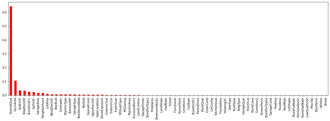
The OverallQual is prescribed a very high feature importance relative to other variables and beyond 9-10 vairables, the importance is negligible. Let’s consider the top 10 variables for modeling using Linear Regression.
from sklearn.linear_model import LinearRegression

from sklearn.model_selection import train_test_split
X_train, X_test, y_train, y_test = train_test_split(X, y, test_size=0.2, random_state=0)

top = pd.Series(dt.feature_importances_, index=X.columns).sort_values(ascending=False)[:10].index.to_list()
reg = LinearRegression().fit(X_train[top],y_train)
print('Training score: {:.2f}'.format(reg.score(X_train[top], y_train)))
print('Testing score: {:.2f}'.format(reg.score(X_test[top], y_test)))
Training score: 0.81
Testing score: 0.62
As you can see, the test score is quite low and our simplified model is not able to properly predict house price and does not improve significantly even by increasing the number of predictors used. Let’s look at the F-stats to see if our coefficent values are statistically significant. Unfortunately, sklearn’s LinearRegression class does not have attributes to display the statistical summary so we use the statsmodels package instead.
import statsmodels.api as sm
from scipy import stats

X2 = sm.add_constant(X_train[top])
est = sm.OLS(y_train, X2)
est2 = est.fit()
print(est2.summary())
                            OLS Regression Results
==============================================================================
Dep. Variable:              SalePrice   R-squared:                       0.814
Model:                            OLS   Adj. R-squared:                  0.812
Method:                 Least Squares   F-statistic:                     506.4
Date:                Fri, 06 Nov 2020   Prob (F-statistic):               0.00
Time:                        18:22:44   Log-Likelihood:                -13839.
No. Observations:                1168   AIC:                         2.770e+04
Df Residuals:                    1157   BIC:                         2.776e+04
Df Model:                          10
Covariance Type:            nonrobust
================================================================================
                   coef    std err          t      P>|t|      [0.025      0.975]
--------------------------------------------------------------------------------
const         -1.07e+05   5017.363    -21.335      0.000   -1.17e+05   -9.72e+04
OverallQual   2.369e+04   1054.524     22.469      0.000    2.16e+04    2.58e+04
GrLivArea       -0.7216     19.581     -0.037      0.971     -39.141      37.697
2ndFlrSF        48.3502     19.957      2.423      0.016       9.193      87.507
TotalBsmtSF     22.6861      4.453      5.094      0.000      13.948      31.424
BsmtFinSF1      24.8870      2.670      9.322      0.000      19.649      30.125
1stFlrSF        51.2961     20.315      2.525      0.012      11.438      91.154
GarageArea      51.5652      6.202      8.314      0.000      39.396      63.734
Neighborhood    67.3986    170.479      0.395      0.693    -267.085     401.882
LotArea          0.4956      0.098      5.042      0.000       0.303       0.688
WoodDeckSF      30.0592      8.263      3.638      0.000      13.848      46.271
==============================================================================
Omnibus:                      312.087   Durbin-Watson:                   2.028
Prob(Omnibus):                  0.000   Jarque-Bera (JB):            21443.147
Skew:                           0.152   Prob(JB):                         0.00
Kurtosis:                      23.989   Cond. No.                     7.71e+04
==============================================================================

Notes:
[1] Standard Errors assume that the covariance matrix of the errors is correctly specified.
[2] The condition number is large, 7.71e+04. This might indicate that there are
strong multicollinearity or other numerical problems.
We see that some of our variables are not significant which means we may need to test other methods of feature selection. The fact that our training Rsq is higher than our test Rsq by a significant amount indicates that we may be overfitting - this calls for Regularization, which we go indepth with in the next post.